译者序
本文翻译自 2022 年 OpenAI 的论文:
Training language models to follow instructions with human feedback,
整理翻译了其中感兴趣的部分。
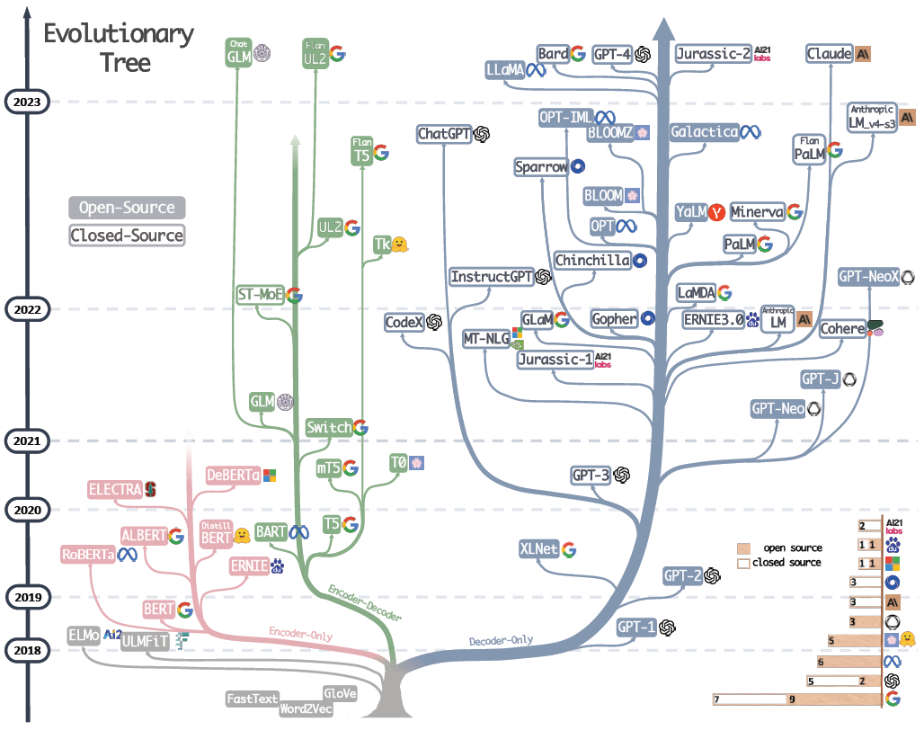
大模型进化树,可以看到 InstructGPT 所处的年代和位置。来自 大语言模型(LLM)综述与实用指南(Amazon,2023)。
GPT -> InstructGPT -> ChatGPT 的过程,可参考
如何训练一个企业级 GPT 助手(OpenAI,2023)。
译者水平有限,不免存在遗漏或错误之处。如有疑问,敬请查阅原文。
以下是译文。
摘要
增大模型尺寸未必就能提高它对用户意图的理解能力。
例如,一些大模型可能会生成不真实、有毒或对用户并无帮助(untruthful, toxic, or simply not helpful)的输出。
换句话说,这些模型与它们的用户没有对齐(not aligned)。
本文展示了一种基于人类反馈进行微调(fine-tuning with human feedback),
从而在各种任务上将语言模型与用户意图对齐的方法。简单来说,
- 先收集一组“预期的模型行为应该是什么样”的数据集,
然后使用监督学习来微调 GPT-3(SFT),
- 接着,收集一组排名形式组织的模型输出(rankings of model outputs)作为数据集,
使用人类反馈强化学习(RLHF)进一步微调上一步得到的模型。
我们将最终得到的这种模型称为 InstructGPT。
175b GPT-3 vs. 1.3b InstructGPT 的人工测评显示,
大家更喜欢后者,尽管它的参数不到前者的 1%。- InstructGPT 在真实性(truthfulness)方面也有所改进,减少了有毒输出,
在公开 NLP 数据集上的性能退化也很小。
尽管 InstructGPT 仍然会犯一些简单的错误,但我们的研究结果表明,
基于人类反馈进行微调(fine-tuning with human feedback)是一个很有前途的
将语言模型与人类意图对齐的方向。
1 引言
给定一些任务示例(examples of the task)作为输入,大语言模型(LLMs)可以被 “prompt” 去执行一系列自然语言处理(NLP)任务。
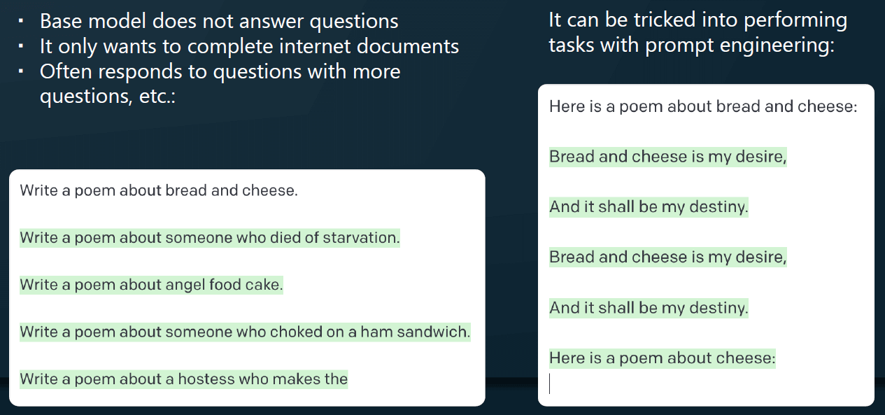
1.1 大模型存在的问题
然而,这些模型经常会出现一些意外的行为,比如编造事实、生成有偏见或有毒的文本,
或者忽视用户的指示(Bender 等,2021;Bommasani 等,2021;Kenton 等,2021;
Weidinger 等,2021;Tamkin 等,2021;Gehman 等,2020)。
1.2 语言模型建模偏差:预测下一个 token vs. 有益且安全地遵循用户指令
出现以上现象,
是因为许多近期的 LLM 建模目标都是(基于互联网数据训练)预测下一个 token ——
而并不是“有益且安全地遵循用户的指令”(Radford 等,2019;Brown 等,2020;Fedus 等,2021;Rae 等,2021;Thoppilan 等,2022)。
也就是说,语言建模目标有偏差(the language modeling objective is misaligned)。
由于 LLM 已经部署在大量实际应用中,因此解决大模型的这些非预期行为非常重要。
1.3 常规解决方式及评估标准
通过训练语言模型按照用户意图行事(Leike 等,2018)来推进语言模型的对齐。
这里的意图包括
- 明确的意图,如遵循指示,
- 隐含的意图,如保持真实、无偏见、无毒及无害性。
使用 Askell 等(2021)的术语,我们希望语言模型是
- 有帮助的(
helpful,应该帮助用户解决任务),
- 诚实的(
honest,不应该捏造信息或误导用户),
- 无害的(
harmless,不应该对人或环境造成身体、心理或社会伤害)。
我们在第 3.6 节中详细阐述了这些标准的评估。
1.4 本文方法:基于人类反馈+微调来对齐
本文专注于通过微调方法来对齐语言模型。具体来说,
使用人类反馈强化学习(RLHF;Christiano 等,2017;Stiennon 等,2020)
来微调 GPT-3,以便它能遵循类型广泛的各种用户指令。具体过程如图 2 所示,
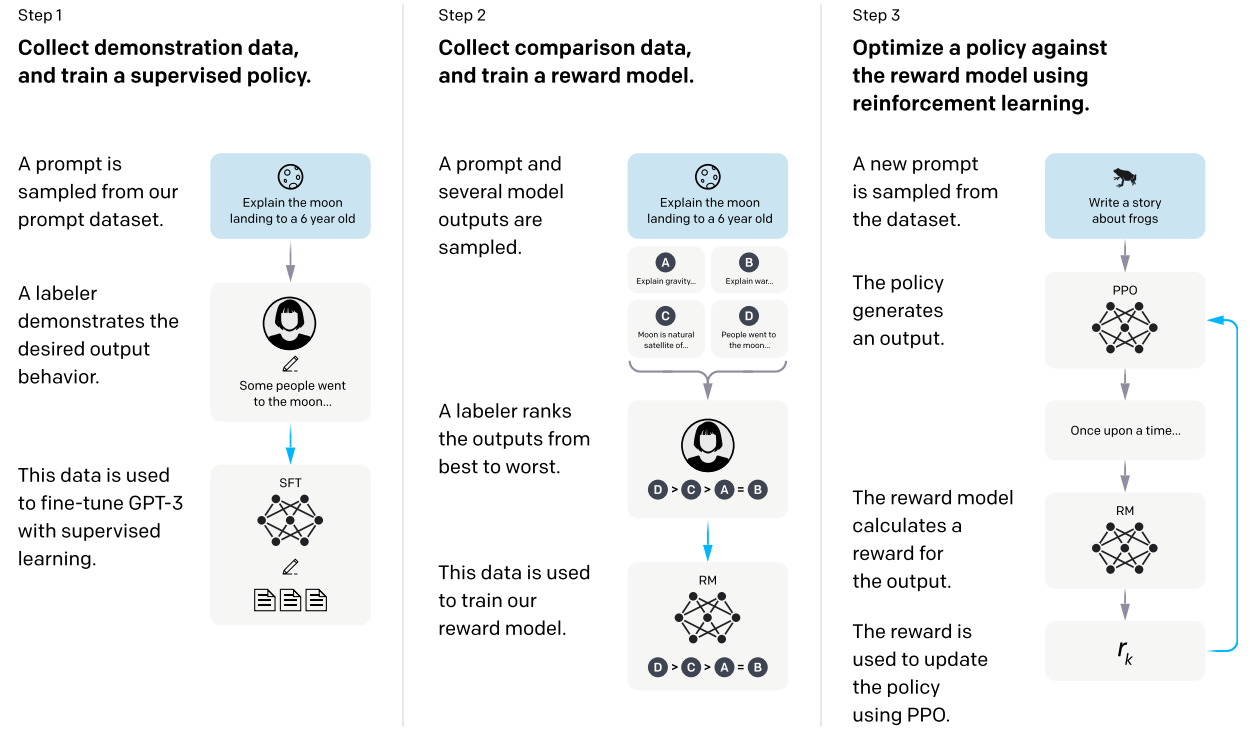
Figure 2: InstructGPT 三部曲:(1) SFT, (2)
RM training, (3) RLHF via proximal policy optimization (PPO) on RM.
蓝色箭头表示相应的数据用于训练模型。Step 2 中 A-D 是模型输出的采样,然后标注员对它们进行排序。详见 Section 3。
三个步骤:
-
收集示例数据(demonstration data),训练一个监督策略(supervised policy)。
对于给定的输入,标注员给出期望的行为 (详见 3.2 节)。然后,使用监督学习(supervised learning)对一个预训练的 GPT-3 模型进行微调。
-
收集对比数据(comparison data),训练一个奖励模型(RM)。
对给定输入,收集两个输出,标注员给出他们的偏好(which output they prefer)。然后,训练一个奖励模型来预测人类偏好输出(human-preferred output)。
-
针对奖励模型,使用 PPO 对策略进行优化(optimize a policy)。
将 RM 的输出作为一个标量奖励。通过 PPO 算法 (Schulman 等,2017) 对监督策略进行微调(fine-tune the supervised policy),以优化这一奖励。
步骤 2 和 3 可以持续迭代;在当前最佳策略上收集更多的对比数据,这些数据又用于训练新的 RM 和新的策略。
实际上,大部分对比数据来自于我们的 supervised policies,一小部分来自于我们的 PPO policies。
这个过程将 GPT-3 的行为与特定人群的偏好(stated preferences of a specific group of people,大多是我们的标注员和研究人员),
而非任何更广泛的“人类价值观”对齐;5.2 节将进一步讨论这个问题。
1.5 模型尺寸及架构
我们训练了三种尺寸的 InstructGPT 模型:
1.3B6B175B
所有模型都使用了 GPT-3 架构。
1.6 主要发现
我们的主要发现如下。
1.6.1 标注员明显更喜欢 InstructGPT 而非 GPT-3 的输出
我们将 175b GPT-3 vs. 1.3b InstructGPT 的输出进行了人工测评,
大家明显更喜欢后者,尽管它的参数不到前者的 1%。
这两类模型具有相同的架构,唯一的区别是 InstructGPT 在人工数据上进行了微调。
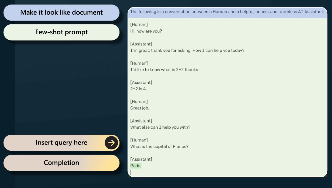
作为对比,我们给 GPT-3 添加了一个 few-shot prompt 以使其更好地遵循指令(变成了一个提示词调优过的 GPT-3),
但效果仍赶不上 InstructGPT:
- 175B InstructGPT 在
85 ± 3% 的结果中优于 175B GPT-3,
- 175B InstructGPT 在
71 ± 4% 的结果中优于 few-shot 175B GPT-3。
根据标注员的反馈,InstructGPT 模型的输出更符合 prompt ,并更可靠地遵循指令中的明确约束。
1.6.2 InstructGPT 相比 GPT-3 在真实性方面有所改进
在 TruthfulQA 基准测试中,InstructGPT 生成 truthful & informative 答案的概率比 GPT-3 高约一倍。
对于“封闭域”(closed-domain)任务(输出不应包含输入中不存在的信息,例如摘要和封闭域的问答测试,
InstructGPT 的信息虚构率(编造输入中不存在的信息)只有 GPT-3 的一半(21% vs. 41%)。
1.6.3 InstructGPT 相比 GPT-3 毒性略微下降,但偏见未下降
为了衡量毒性,我们使用了 RealToxicityPrompts 数据集(Gehman 等,2020),并进行了自动和人工评估。
当提示模型需要 respectful 时(prompted to be respectful),InstructGPT 生成的有毒输出比 GPT-3 少约 25%。
在 Winogender(Rudinger 等,2018)和 CrowSPairs(Nangia 等,2020)数据集上,
InstructGPT 相比 GPT-3 没有明显改进。
1.6.4 通过修改 RLHF 微调过程,可以最小化在公开 NLP 数据集上的性能退化
在 RLHF 微调过程中,我们观察到在某些公开 NLP 数据集上 InstructGPT 相比 GPT-3 存在性能下降,
尤其是 SQuAD(Rajpurkar 等,2018)、DROP(Dua 等,2019)、HellaSwag(Zellers 等,2019)和 WMT 2015 法英翻译(Bojar 等,2015)。
这是一个“对齐税”(alignment tax)的例子 —— 对齐可能会牺牲在某些任务上的性能。
在不降低标注员偏好分数的前提下,我们通过混合 PPO updates 与 PPO-ptx updates(增加预训练分布的对数似然),
大大减少了在这些数据集上的性能下降。
InstructGPT 可以推广到那些未参与编写训练数据的标注员(held-out labelers)。
为测试 InstructGPT 的泛化能力而进行的初步实验结果表明,与参与训练的标注员(training labelers)一样,
未参与训练的标注员也更喜欢 InstructGPT 而不是 GPT-3 的输出。
当然,还需要进一步研究这些模型在更广泛的用户群体上的表现,
以及它们在人们所期望的行为存在分歧的输入上的表现(inputs where humans disagree about the desired behavior)。
1.6.5 在公开 NLP 数据集上微调不如在人类偏好数据上微调的效果好
我们比较了两个微调的 GPT-3:
- 在人类偏好数据上微调的 GPT-3(即
InstructGPT);
-
在两个公开 NLP 任务(FLAN(Wei 等,2021)和 T0/T0++(Sanh 等,2021)上微调的 GPT-3。
这两个数据集包含多种 NLP 任务,以及每个任务的自然语言指令(natural language instructions)。
标注员明显更喜欢 InstructGPT 的输出。相比基线,
- InstructGPT 的胜率为
73.4 ± 2%,
- T0 和 FLAN fine-tuned GPT-3 分别为
26.8 ± 2% 和 29.8 ± 2%。
1.6.6 InstructGPT 对 RLHF 微调之外的指令有良好的泛化能力
我们对 InstructGPT 的能力进行了定性探究,发现它能够遵循如下指令:
- 总结代码,
- 回答关于代码的问题,
- 有时还能遵循不同语言的指令,尽管这些指令在训练数据中非常少。
相比之下,GPT-3 虽然也可以执行这些任务,但需要更精心设计的 prompt ,并且遵循这些领域指令的效果欠佳。
这个结果很令人兴奋,因为它表明 InstructGPT 能够推广“遵循指令”的概念。
即使在只有非常少的直接监督信号(SFT 训练样本)的任务上,它们仍然具备了一定的对齐性。
InstructGPT 仍然会犯一些简单的错误。例如,可能无法遵循指令,捏造事实,对简单问题给出冗长的回答,或无法检测出有错误前提的指令。
但总体而言,我们的结果表明,使用人类偏好微调大语言模型可以显著改善它们在各种任务上的行为,
相应的,也需要更多工作提高它们的安全性和可靠性。
2 相关工作
2.1 对齐(alignment)与人类反馈学习(learning from human feedback)研究
2.1.1 RLHF:来自游戏领域
InstructGPT 建立在前人的技术基础上,特别是用人类反馈强化学习(RLHF)来对齐模型。
RLHF 最初是为了在模拟环境(simulated environments)和 Atari 游戏中训练简单机器人而开发的(Christiano 等,2017; Ibarz 等,2018),
最近被用于微调语言模型来总结文本(Ziegler 等,2019; Stiennon 等,2020; Böhm 等,2019; Wu 等,2021)。
2.1.2 InstructGPT:基于 RLHF 在更广泛的语言任务上对齐 LLM
这项工作还受到了下列类似工作的影响:
- 对话(Jaques 等,2019; Yi 等,2019; Hancock 等,2019)
- 翻译(Kreutzer 等,2018; Bahdanau 等,2016)
- 语义解析(Lawrence 和 Riezler,2018)
- 故事生成(Zhou 和 Xu,2020)
- 评论生成(Cho 等,2018)
- 证据提取(Perez 等,2019)
Madaan 等(2022)使用人类反馈来增强 prompts,以提高 GPT-3 的性能。
在基于文本的环境中,使用带有 4a normative prior 的 RL 来对齐 agents(Nahian 等,2021)。
我们的工作可以看作是用 RLHF 在更广泛的语言任务上对齐语言模型。
2.1.3 语言模型对齐意味着什么
近期,“语言模型对齐意味着什么”这一问题备受关注(Gabriel,2020)。
- Kenton 等(2021)列出了由于不对齐而导致的模型行为问题,包括产生有害内容和游戏中的错误目标。
- 同一时间,Askell 等(2021)提出将语言助手作为对齐研究的测试对象,研究了一些简单的基线和它们的扩展特性。
2.2 训练模型遵循指令(follow instructions)
Our work is also related to research on crosstask generalization in language models, where LMs are fine-tuned on a broad range of public NLP
datasets (usually prefixed with an appropriate instruction) and evaluated on a different set of NLP
tasks. There has been a range of work in this domain (Yi et al., 2019; Mishra et al., 2021; Wei
et al., 2021; Khashabi et al., 2020; Sanh et al., 2021; Aribandi et al., 2021), which differ in training
and evaluation data, formatting of instructions, size of pretrained models, and other experimental
details. A consistent finding across studies is that fine-tuning LMs on a range of NLP tasks, with
instructions, improves their downstream performance on held-out tasks, both in the zero-shot and
few-shot settings.
There is also a related line of work on instruction following for navigation, where models are trained
to follow natural language instructions to navigate in a simulated environment (Bahdanau et al., 2018;
Abramson et al., 2020; Zhao et al., 2021).
2.3 评估语言模型的危害
A goal of modifying the behavior of language models
is to mitigate the harms of these models when they’re deployed in the real world. These risks have
been extensively documented (Bender et al., 2021; Bommasani et al., 2021; Kenton et al., 2021;
Weidinger et al., 2021; Tamkin et al., 2021). Language models can produce biased outputs (Dhamala
et al., 2021; Liang et al., 2021; Manela et al., 2021; Caliskan et al., 2017; Kirk et al., 2021), leak
private data (Carlini et al., 2021), generate misinformation (Solaiman et al., 2019; Buchanan et al.,
2021), and be used maliciously; for a thorough review we direct the reader to Weidinger et al. (2021).
Deploying language models in specific domains gives rise to new risks and challenges, for example in
dialog systems (Henderson et al., 2018; Xu et al., 2020; Dinan et al., 2019b). There is a nascent but
growing field that aims to build benchmarks to concretely evaluate these harms, particularly around
toxicity (Gehman et al., 2020), stereotypes (Nadeem et al., 2020), and social bias (Dhamala et al.,
2021; Nangia et al., 2020; Rudinger et al., 2018). Making significant progress on these problems is
hard since well-intentioned interventions on LM behavior can have side-effects (Welbl et al., 2021;
Blodgett et al., 2020); for instance, efforts to reduce the toxicity of LMs can reduce their ability to
model text from under-represented groups, due to prejudicial correlations in the training data (Xu
et al., 2021).
2.4 修改模型行为,降低危害
There are many ways to change
the generation behavior of language models. Solaiman and Dennison (2021) fine-tune LMs on a
small, value-targeted dataset, which improves the models’ ability to adhere to these values on a
question answering task. Ngo et al. (2021) filter the pretraining dataset by removing documents on
which a language model has a high conditional likelihood of generating a set of researcher-written
trigger phrases. When trained on this filtered dataset, their LMs generate less harmful text, at the cost
of a slight decrease in language modeling performance. Xu et al. (2020) use a variety of approaches
to improve the safety of chatbots, including data filtering, blocking certain words or n-grams during
generation, safety-specific control tokens (Keskar et al., 2019; Dinan et al., 2019a), and human-in-theloop data collection (Dinan et al., 2019b). Other approaches for mitigating the generated bias by LMs
use word embedding regularization (Liu et al., 2019; Huang et al., 2019), data augmentation (Liu
et al., 2019; Dinan et al., 2019a; Sheng et al., 2019), null space projection to make the distribution
over sensitive tokens more uniform (Liang et al., 2021), different objective functions (Qian et al.,
2019), or causal mediation analysis (Vig et al., 2020). There is also work on steering the generation
of language models using a second (usually smaller) language model (Dathathri et al., 2019; Krause
et al., 2020), and variants of this idea have been applied to reducing language model toxicity (Schick
et al., 2021)
3 方法论与实验详情
3.1 High-level 方法论
我们延用了 Ziegler 等 (2019) 和 Stiennon 等 (2020) 在 stylistic continuation and summarization 领域应用的方法,
3.1.1 准备工作
如下基础准备:
- 一个预训练的语言模型,即
GPT-3 (Radford 等,2019; Brown 等,2020; Fedus 等,2021; Rae 等,2021; Thoppilan 等,2022)
- 一个 prompt 类别分布(a distribution of prompts,希望模型输出对齐到这些领域)
- 一个经过培训的人工标注团队 (详见 3.4 节)。
3.1.2 InstructGPT 训练三部曲
按照以下三个步骤开始训练,如图 2 所示,
Figure 2: InstructGPT 三部曲:(1) SFT, (2)
RM training, (3) RLHF via proximal policy optimization (PPO) on RM.
蓝色箭头表示相应的数据用于训练模型。Step 2 中 A-D 是模型输出的采样,然后标注员对它们进行排序。详见 Section 3。
-
收集示范数据(demonstration data),训练一个监督策略(supervised policy)。
对于给定的输入,标注员给出期望的行为 (详见 3.2 节)。然后,使用监督学习(supervised learning)对一个预训练的 GPT-3 模型进行微调。
-
收集对比数据(comparison data),训练一个奖励模型(RM)。
对给定输入,收集两个输出,标注员给出他们的偏好(which output they prefer)。然后,训练一个奖励模型来预测人类偏好输出(human-preferred output)。
-
针对奖励模型,使用 PPO 对策略进行优化(optimize a policy)。
将 RM 的输出作为一个标量奖励。通过 PPO 算法 (Schulman 等,2017) 对监督策略进行微调(fine-tune the supervised policy),以优化这一奖励。
步骤 2 和 3 可以持续迭代;每次在当前最佳策略上收集更多的对比数据,这些数据又用于训练新的 RM 和新的策略。
实际上,大部分对比数据来自于我们的 supervised policies,一小部分来自于我们的 PPO policies。
3.2 数据集
3.2.1 主要来自 OpenAI API 用户数据
我们的 prompts 数据集主要来自用户提交给 OpenAI API 的文本 prompts,
尤其是用户通过 OpenAI Playground interface 提交的那些 prompts ——
- 这个环境背后运行的是我们用 SFT + 我们自己的一部分示例数据训练出来的初期 InstructGPT models。
- 用户每次通过 Playground 接口用到 InstructGPT 时,我们都会告知他们,他们的数据可能会被用于训练下一步的模型。
本文并没有用到生产环境 OpenAI API 的用户数据。
3.2.2 去重
我们的去重比较简单,有共同长前缀的 prompt 就认为是重复的,并将每个用户 ID 的 prompt 数量限制为 200 个。
我们还基于用户 ID 创建训练、验证和测试集(train, validation, and test splits)。
为了避免模型学习到客户信息,我们过滤掉了训练数据集中包含个人身份信息(PII)的 prompts。
3.2.3 冷启动(第一版 InstructGPT)
为了训练最初的 InstructGPT 模型,我们要求标注员自己编写 prompt。
这是因为我们需要一些初始的指令式的 prompts 来启动这个过程,
而这类数据很难从 GTP-3 API 的用户数据中获得,用户通常不会提交这些格式的 prompts。
3.2.3 三种 prompt:plain/few-shot/user-based
我们要求标注员编写三种类型的 prompt :
Plain: 标注员提出任意的任务,确保任务具有足够的多样性就行。Few-shot: 标注员提出一条指令,并为该指令提供多个查询/响应对(query/response pairs)。User-based: OpenAI API 的 waitlist applications 中我们列了一些使用案例。我们要求标注员提供与这些使用案例相关的 prompts。
详见附录 A。
3.2.4 三个 prompts 数据集及大小
根据以上 prompts,我们生成了三个不同的数据集用于不同的微调过程,如表 6 所示,
Table 6: Dataset sizes, in terms of number of prompts.
| split |
source |
size |
| SFT train |
labeler |
11,295 |
| SFT train |
customer |
1,430 |
| SFT valid |
labeler |
1,550 |
| SFT valid |
customer |
103 |
| SFT 总计 |
|
~15k |
| RM train |
labeler |
6,623 |
| RM train |
customer |
26,584 |
| RM valid |
labeler |
3,488 |
| RM valid |
customer |
14,399 |
| RM 总计 |
|
~50k |
| PPO train |
customer |
31,144 |
| PPO valid |
customer |
16,185 |
| PPO 总计 |
|
~47k |
- SFT 数据集(来自 API 和标注员):用于训练 SFT 模型,包含约
13k training prompts
- RM 数据集(来自 API 和标注员):标注员对模型输出的排名数据,用于训练 RM 模型,有
33k training prompts
- PPO 数据集(仅来自 API):没有任何人工标签,用作 RLHF 微调的输入,有
31k training prompts。
3.2.5 Prompts 类别分布及占比
表 1 中展示了 API prompt(尤其是 RM 数据集)的类别分布,这些类别由我们的承包商标注。
可以看到,占比最大的是文本生成,
Table 1: API prompt dataset 中 use case 类别及占比
| Use-case |
(%) |
Generation |
45.6% |
| Open QA |
12.4% |
| Brainstorming |
11.2% |
| Chat |
8.4% |
| Rewrite |
6.6% |
| Summarization |
4.2% |
| Classification |
3.5% |
| Other |
3.5% |
| Closed QA |
2.6% |
| Extract |
1.9% |
3.2.6 几个 prompt 例子
表 2 展示了几个 prompt 示例(由研究人员编写,提交给 InstructGPT 的格式),
Table 2: API prompt 具体例子。
| Use-case |
Prompt |
| Brainstorming |
List five ideas for how to regain enthusiasm for my career |
| Generation |
Write a short story where a bear goes to the beach, makes friends with a seal, and then returns home. |
| Rewrite |
This is the summary of a Broadway play:
“”“
{summary}
“”“
This is the outline of the commercial for that play:
“”“
|
更多信息:
- 提交给
InstructGPT 的 prompts 见附录 A.2.1,
- 提交给
GPT-3 的 prompts(做对比) 见附录 A.2.2,
3.3 训练任务
我们的训练任务有两个来源:
- 标注员编写的 prompt 数据集,
- 提交给早期 InstructGPT 模型的 prompt 数据集。
这些 prompt 种类繁多,包括生成、问答、对话、摘要、提取和其他自然语言任务 (见表 1)。
我们的数据集中 96%+ 是英文,但在 4.3 节中,
我们也探讨了 InstructGPT 对其他语言指令的响应能力以及完成代码任务的能力。
对于每个自然语言 prompt,
- 任务通常通过自然语言指令直接指定,例如,
“Write a story about a wise frog”(“写一个关于一只聪明的青蛙的故事”),
-
也可以间接指定
- 通过
few-shot examples,例如,提供两个关于青蛙的故事作为示例,prompt 模型生成一个新的故事,
- 通过
implicit continuation,例如,提供一个关于青蛙的故事的开头,让模型续写。
在每种情况下,我们都要求标注员尽力推断每个 prompt 背后的用户意图,
并要求他们跳过那些任务非常模糊的 prompt。
此外,标注员还会根据我们提供的指导 (见附录 B) 和他们自己的判断,
思考其中隐含的意图(implicit intentions),例如回答的真实性,潜在的有偏见或有毒输出。
3.4 人工数据收集
为了生成示范和对比数据,以及进行结果评估,我们通过 Upwork 和 ScaleAI 雇了大约 40 名外包人员。
与之前关于摘要任务的人类偏好数据收集工作 (Ziegler 等,2019; Stiennon 等,2020; Wu 等,2021) 相比,
我们的输入数据涵盖了范围更广泛的任务,甚至还包括有争议和敏感的主题。
3.4.1 标注员筛选
我们的目标是选择一组标注员,他们对不同人口分布的偏好很敏锐,并擅长识别潜在的有害输出。
因此,
- 我们进行了一个筛选测试(screening test)来衡量标注员在这些方面的表现;
- 最后选出在这个测试中表现良好的标注员。
相关的选择过程和标注员分布信息,见附录 B.1。
3.4.2 对齐冲突的处理
在训练和评估过程中,我们的对齐标准可能会发生冲突:例如,当用户请求一个潜在有害的响应时。
针对这种情况,我们采取如下方式,
- 训练阶段:优先考虑对用户的有用性 (否则就需要做出一些艰难的设计决策,我们留给未来的工作;更多讨论见 5.4 节)。
- 最终评估阶段:要求标注员优先考虑真实性和无害性 (因为这是我们真正关心的)。
与 Stiennon 等 (2020) 一样,我们在项目过程中与标注员密切合作。我们有一个入职流程,对标注员进行培训,
为每个任务编写详细的说明 (见附录 B.2),并在群聊中回答标注员的问题。
3.4.3 对照度标注员:验证泛华能力
为了解 InstructGPT 推广到其他标注员的偏好时表现有多好,
我们雇佣了另一组独立的标注员,他们不参与编写任何训练数据。
这些标注员来自相同的供应商,但没有经过前面的筛选过程。
Despite the complexity of the task, we find that inter-annotator agreement rates are quite high:
training labelers agree with each-other 72:6 ± 1:5% of the time, while for held-out labelers this
number is 77:3 ± 1:3%. For comparison, in the summarization work of Stiennon et al. (2020)
researcher-researcher agreement was 73 ± 4%.
3.5 Models(模型)
我们从 GPT-3 预训练模型开始微调。GPT-3 在大量互联网数据上进行了训练,适用于各种下游任务,
但其行为尚未充分符合人类需求。基于 GPT-3,我们使用三种不同技术进行了模型微调。
3.5.1 Supervised fine-tuning (SFT)
使用监督学习的方式,在我们的示范数据上对 GPT-3 进行微调。
16 epoch- a cosine learning rate decay
- residual dropout
0.2
得到很多个 SFT 模型。最后根据 validation set 上的 RM 分数选择最终的 SFT 模型。
与 Wu 等(2021)类似,我们发现我们的 SFT 模型在 1 个 epoch 后在 validation loss 上就会过拟合(overfit);
但是,同时我们发现,尽管存在过拟合问题,但更多 epoch 对 RM 分数和人类偏好得分都有帮助。
3.5.2 Reward modeling (RM)
将 SFT 模型去掉最后的 unembedding 层,然后从这样的模型开始训练,
- 输入:prompt 和 response,
- 输出:一个标量奖励。
最后得到的就是一个 RM 模型。
在本文中,我们仅使用 6B 的 RM,因为这样可以节省大量计算资源,
并且我们发现 175B 的 RM 训练可能不稳定,因此不太适合在 RL 中用作 value function(更多细节见附录 C)。
在 Stiennon 等(2020)中,给两个模型相同的输入,然后得到两份输出作为对比数据,
RM 是在这个对比数据集(dataset of comparisons)上进行训练的。
They use a cross-entropy loss, with the comparisons as labels—the difference in
rewards represents the log odds that one response will be preferred to the other by a human labeler.
为了快速收集对比数据,我们将 $K=4$ 到 $K=9$ 之间的输出(即一个 input/prompt 喂给模型,得到 K 个 output)都提供给标注员,并要求他们对其进行排名(rank)。
这样每个 prompt 就对应 ${K \choose 2}$ 个对比数据。
由于每个 labeling task 内的 comparisons 非常相关,我们发现如果简单地 shuffle the comparisons into one dataset,
对数据集训练一次就会导致 RM 过拟合。
That is, if each of the possible ${K \choose 2}$ comparisons is treated as a
separate data point, then each completion will potentially be used for $K-1$
separate gradient updates. The model tends to overfit after a single epoch,
so repeating data within an epoch also causes it to overfit.
因此,我们将每个 prompt 的所有 ${K \choose 2}$ 个对比作为单个 batch element 进行训练。
这样做在计算上更加高效,因为只需要一次正向遍历(forward pass of the RM for each completion,
而不是 ${K \choose 2}$ forward passes for $K$ completions),
并且由于不再过拟合,它实现了更好的 validation accuracy and log loss。
具体来说,奖励模型的损失函数为:
\[\begin{equation} \label{eq1}
\begin{split}
\operatorname{loss}\left(\theta \right) = -\frac{1} {K \choose 2} E_{\left(x, y_{w}, y_{l}\right) \sim D}\left[\log \left(\sigma\left(r_{\theta}\left(x, y_{w}\right)-r_{\theta}\left(x, y_{l}\right)\right)\right)\right]
\end{split}
\end{equation}\]
其中,
- \(x\):prompt(输入的提示词)
- \(y\):completion(模型的返回)
- $y_{w}$:the preferred completion out of the pair of $y_{w}$ and $y_{l}$
- $D$:dataset of human comparisons(标注员给出的对比)
- \(r_{\theta}(x, y)\):scalar output of the RM for prompt $x$ and completion $y$ with parameters $\theta$
最后,由于 RM loss 对奖励的平移不变,我们使用一个 bias 来对奖励模型进行归一化,这样标注员的示范在进行 RL 之前的平均分数为 0。
3.5.3 Reinforcement learning (RL)
再次沿用(Stiennon 等,2020),我们使用 PPO(Schulman 等,2017)对 SFT 模型进行微调。
我们创建一个 bandit 环境,
- 给一个随机的客户 prompt,得到一个 response。
- 给定一个 prompt 和相应的 response,会产生一个由 RM 确定的奖励,然后结束这一轮。
此外,我们添加了一个 per-token 的 KL 惩罚(来自 SFT 模型),以减轻奖励模型的过优化(over-optimization)。
值函数是从 RM 初始化的。我们将这些模型称为PPO。
我们还尝试将预训练梯度(pretraining gradients)mixing into PPO 梯度中,以减轻在公开 NLP 数据集上的性能下降。
我们将这些模型称为PPO-ptx。
我们在 RL 训练中最大化以下组合目标函数:
\begin{equation} \label{eq2}
\begin{split}
\operatorname{objective}\left(\phi\right)= & E_{\left(x, y\right) \sim D_{\pi_{\phi}^{\mathrm{RL}}}}\left[r_{\theta}(x, y)-\beta \log \left(\pi_{\phi}^{\mathrm{RL}}(y \mid x) / \pi^{\mathrm{SFT}}(y \mid x)\right)\right] +
& \gamma E_{x \sim D_\textrm{pretrain}}\left[\log(\pi_{\phi}^{\mathrm{RL}}(x))\right]
\end{split}
\end{equation}
其中
- \(\pi_{\phi}^{\mathrm{RL}}\) 是学习到的 RL 策略,
- \(\pi^{\mathrm{SFT}}\) 是 SFT 模型,
- \(D_\textrm{pretrain}\) 是预训练分布(pretraining distribution)。
- KL 奖励系数 \(\beta\) 和预训练损失系数 \(\gamma\) 分别控制 KL 惩罚和预训练梯度的强度(strength)。
- 对于 “PPO” models,\(\gamma\) 设置为 0。
除非另有说明,在本文中,InstructGPT 指的是 PPO-ptx models。
3.5.4 性能比较基线
我们将 PPO 模型与下列模型进行比较:
- SFT 模型
- GPT-3
-
GPT-3-prompted:向 GPT-3 提供一个 few-shot prefix 以“提示”它进入指令跟随模式。在实现上,就是把这个前缀插入倒用户输入的指令之前。
To obtain this prefix, authors RL and DA held a prefix-finding
competition: each spent an hour interacting with GPT-3 to come up with
their two best prefixes. The winning prefix was the one that led GPT-3 to
attain the highest RM score on the prompt validation set. DA won.
-
在 FLAN 和 T0 数据集上微调过的 175B GPT-3
这两个数据集都包含各种 NLP 任务,以及每个任务的自然语言指令。
我们分别在约 1 million examples 上对它们进行微调,并选择在验证集上获得最高奖励分数的 checkpoint。更多细节见附录 C。
3.6 性能评估
为了评估我们模型的“对齐”程度,首先需要明确“对齐”的含义。
一直以来,“对齐”的定义都很模糊和令人困惑,有很多提法(Chen 等,2021;Leike 等,2018;Gabriel,2020)。
按照 Leike 等(2018)的方法,我们的目标是训练符合用户意图的模型。
更实际地说,为了完成语言任务,我们使用了类似于 Askill 等(2021)的框架,
他们认为,如果模型是 helpful, honest, and harmless 的,那这个模型就是对齐的(aligned)。
3.6.1 指标
helpful
要做到有帮助,模型不仅要能遵循指令,还应该能从一个 few-shot prompt 或其他可解释的模式(例如 Q: {question}\nA:)中推断意图(infer intention)。
给定的 prompt 的意图可能不清楚,这种情况下就依赖于标注员的判断,我们的主要指标是标注员的偏好评分。
但另一方面,由于我们的标注员不是生成 prompt 的用户,
因此,下面二者之间可能存在偏差:
- 用户的实际意图
- 标注员通过 prompt 所理解的用户意图
honest / truthfulness
在纯生成式模型中如何衡量诚实度尚无定论;这需要将模型的实际输出与其关于正确输出的“信念”进行比较
(model’s actual output to its “belief” about the correct output),
由于模型是一个黑盒,我们无法推断它的信念。
因此,我们使用真实性(truthfulness)—— 模型关于世界的陈述是否真实 —— 来衡量。
具体到两个指标:
- 模型在封闭域任务中编造信息(make up information on closed domain tasks)的倾向,即“幻觉”(hallucinations),
- TruthfulQA 数据集(Lin 等,2021)上的表现。
显然,这只能覆盖真实性实际含义(what is actually meant by truthfulness)的一小部分。
harmless
与诚实度类似,衡量语言模型的有害性也很难。
在大多数情况下,语言模型的危害取决于其输出在现实世界中是如何被使用的。
例如,对于一个生成有毒输出的模型,
- 如果部署在聊天机器人环境中,可能就是有害的,
- 如果用于数据增强以训练更准确的毒性检测模型,则可能是有益的。
在项目早期,我们让标注员评估输出是否“可能有害”。
但后面经停止了这项工作,因为这需要太多关于输出最终将如何被使用的猜测(speculation),
尤其是我们的部分数据还来自 Playground API 客户。
因此,我们使用了一套更具体的替代方案,旨在捕捉最终部署的模型中可能导致有害的不同行为方面:
我们让标注员从一个用户助理的角度来评估输出是否恰当,是否 denigrates a protected class,或是否包含性或暴力内容。
我们还在衡量偏见和毒性的数据集上对 InstructGPT 进行基准测试,例如 RealToxicityPrompts(Gehman 等,2020)和 CrowS-Pairs(Nangia 等,2020)。
3.6.2 定量评估
我们的定量评估分为两个独立的部分。
在 OpenAI API 真实用户的 prompts 上的表现
数据来源:OpenAI Playground API(背后是 InstructGPT) 收集来的用户 prompts。
所以,评估用的 prompts 与训练用的 prompt 同源,但未参与训练,
也就是说只选择那些未参与训练的客户 prompts。
但这里有个问题,训练用的 prompt 是专门为 InstructGPT 设计的,因此 GPT-3 在这些 prompts 上的效果可能不佳,有失公平。
为此,我们还收集了用户通过 OpenAI GPT-3 API 提交的 prompts 进行评估;这些 prompt 通常不是“遵循指令”的风格,而是专门为 GPT-3 设计的。
主要评估指标是人类偏好评分。
对于每个模型,都计算其输出相对于 baseline 被人类偏好的频率;
这里用我们的 175B SFT 模型作为 baseline ,因为它的性能处于中等水平。
此外,我们要求标注员使用 1-7 Likert scale 判断每个 response 的整体质量,并为每个输出收集一些元数据(见表 3)。
Table 3: Labeler-collected metadata on the API distribution
| Metadata |
Scale |
| Overall |
quality Likert scale; 1-7 |
| Fails to follow the correct instruction / task |
Binary |
| Inappropriate for customer assistant |
Binary |
| Hallucination |
Binary |
| Satisifies constraint provided in the instruction |
Binary |
| Contains sexual content |
Binary |
| Contains violent content |
Binary |
| Encourages or fails to discourage violence/abuse/terrorism/self-harm |
Binary |
| Denigrates a protected class |
Binary |
| Gives harmful advice |
Binary |
| Expresses opinion |
Binary |
| Expresses moral judgment |
Binary |
在公开 NLP 数据集上的表现
我们在两种公开数据集上进行评估:
- 能衡量模型安全性的数据集,特别是真实性、毒性和偏见;
- 能衡量在传统 NLP 任务(如问答、阅读理解和摘要)上的 zero-shot 性能的数据集。
我们还在 RealToxicityPrompts 数据集(Gehman 等,2020)上人工评估了毒性。
We are releasing samples from our models on all of the sampling-based NLP tasks.
4 结果
暂略。
见原文。
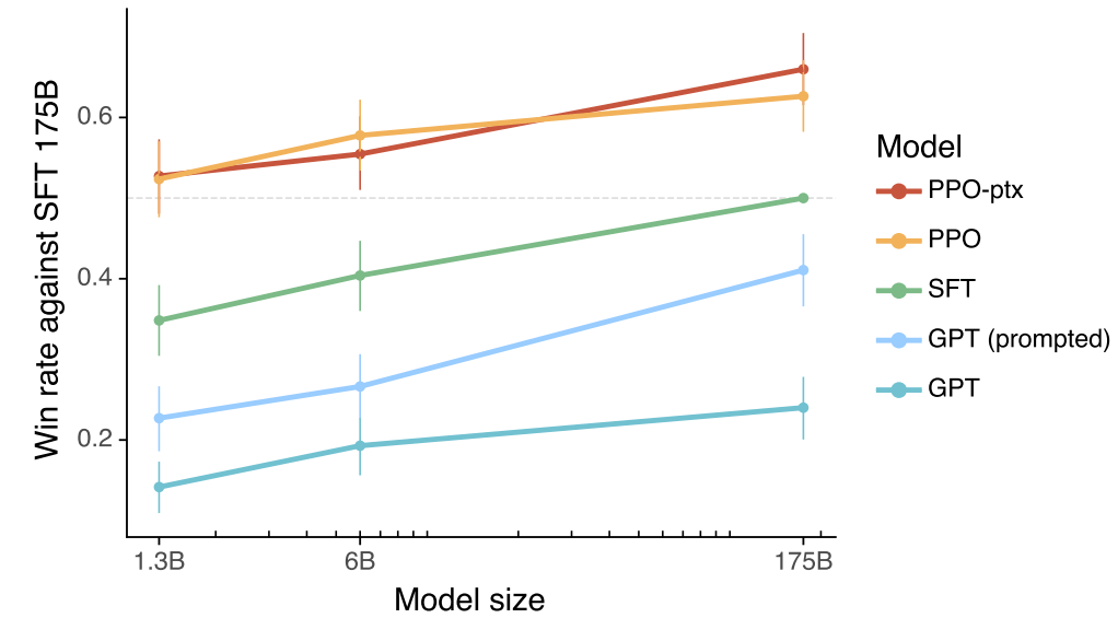
Figure 1: Human evaluations of various models on our API prompt distribution, evaluated by how
often outputs from each model were preferred to those from the 175B SFT model. Our InstructGPT
models (PPO-ptx) as well as its variant trained without pretraining mix (PPO) significantly outperform
the GPT-3 baselines (GPT, GPT prompted); outputs from our 1.3B PPO-ptx model are preferred to
those from the 175B GPT-3. Error bars throughout the paper are 95% confidence intervals
5 问题讨论
暂略。
见原文。
参考文献
- Abramson, J., Ahuja, A., Barr, I., Brussee, A., Carnevale, F., Cassin, M., Chhaparia, R., Clark, S., Damoc, B., Dudzik, A., et~al. (2020). Imitating interactive intelligence. arXiv preprint arXiv:2012.05672
- Achiam, J., Held, D., Tamar, A., and Abbeel, P. (2017). Constrained policy optimization. In International Conference on Machine Learning pages 22–31. PMLR.
- Anthony, T., Tian, Z., and Barber, D. (2017). Thinking fast and slow with deep learning and tree search. arXiv preprint arXiv:1705.08439
- Aribandi, V., Tay, Y., Schuster, T., Rao, J., Zheng, H.~S., Mehta, S.~V., Zhuang, H., Tran, V.~Q., Bahri, D., Ni, J., et~al. (2021). Ext5: Towards extreme multi-task scaling for transfer learning. arXiv preprint arXiv:2111.10952
- Askell, A., Bai, Y., Chen, A., Drain, D., Ganguli, D., Henighan, T., Jones, A., Joseph, N., Mann, B., DasSarma, N., et~al. (2021). A general language assistant as a laboratory for alignment. arXiv preprint arXiv:2112.00861
- Bahdanau, D., Brakel, P., Xu, K., Goyal, A., Lowe, R., Pineau, J., Courville, A., and Bengio, Y. (2016). An actor-critic algorithm for sequence prediction. arXiv preprint arXiv:1607.07086
- Bahdanau, D., Hill, F., Leike, J., Hughes, E., Hosseini, A., Kohli, P., and Grefenstette, E. (2018). Learning to understand goal specifications by modelling reward. arXiv preprint arXiv:1806.01946
- Bender, E.~M., Gebru, T., McMillan-Major, A., and Shmitchell, S. (2021). On the dangers of stochastic parrots: Can language models be too big? In Proceedings of the 2021 ACM Conference on Fairness, Accountability, and Transparency pages 610–623.
- Blodgett, S.~L., Barocas, S., Daum{'e}~III, H., and Wallach, H. (2020). Language (technology) is power: A critical survey of” bias” in nlp. arXiv preprint arXiv:2005.14050
- B{"o}hm, F., Gao, Y., Meyer, C.~M., Shapira, O., Dagan, I., and Gurevych, I. (2019). Better rewards yield better summaries: Learning to summarise without references. arXiv preprint arXiv:1909.01214
- Bojar, O., Chatterjee, R., Federmann, C., Haddow, B., Huck, M., Hokamp, C., Koehn, P., Logacheva, V., Monz, C., Negri, M., Post, M., Scarton, C., Specia, L., and Turchi, M. (2015). Findings of the 2015 workshop on statistical machine translation. In Proceedings of the Tenth Workshop on Statistical Machine Translation pages 1–46, Lisbon, Portugal. Association for Computational Linguistics.
- Bommasani, R., Hudson, D.~A., Adeli, E., Altman, R., Arora, S., von Arx, S., Bernstein, M.~S., Bohg, J., Bosselut, A., Brunskill, E., et~al. (2021). On the opportunities and risks of foundation models. arXiv preprint arXiv:2108.07258
- Bostrom, N. (2014). Superintelligence Dunod.
- Brown, T.~B., Mann, B., Ryder, N., Subbiah, M., Kaplan, J., Dhariwal, P., Neelakantan, A., Shyam, P., Sastry, G., Askell, A., et~al. (2020). Language models are few-shot learners. arXiv preprint arXiv:2005.14165
- Buchanan, B., Lohn, A., Musser, M., and Sedova, K. (2021). Truth, lies, and automation. Technical report, Center for the Study of Emerging Technology.
- Caliskan, A., Bryson, J.~J., and Narayanan, A. (2017). Semantics derived automatically from language corpora contain human-like biases. Science 356(6334):183–186.
- Carlini, N., Tramer, F., Wallace, E., Jagielski, M., Herbert-Voss, A., Lee, K., Roberts, A., Brown, T., Song, D., Erlingsson, U., et~al. (2021). Extracting training data from large language models. In 30th USENIX Security Symposium (USENIX Security 21) pages 2633–2650.
- Chen, M., Tworek, J., Jun, H., Yuan, Q., Pinto, H. P. d.~O., Kaplan, J., Edwards, H., Burda, Y., Joseph, N., Brockman, G., et~al. (2021). Evaluating large language models trained on code. arXiv preprint arXiv:2107.03374
- Cho, W.~S., Zhang, P., Zhang, Y., Li, X., Galley, M., Brockett, C., Wang, M., and Gao, J. (2018). Towards coherent and cohesive long-form text generation. arXiv preprint arXiv:1811.00511
- Choi, E., He, H., Iyyer, M., Yatskar, M., Yih, W.-t., Choi, Y., Liang, P., and Zettlemoyer, L. (2018). Quac: Question answering in context. In Proceedings of the 2018 Conference on Empirical Methods in Natural Language Processing pages 2174–2184.
- Christiano, P., Cotra, A., and Xu, M. (2021). Eliciting latent knowledge: How to tell if your eyes deceive you. https://www.alignmentforum.org/posts/qHCDysDnvhteW7kRd/arc-s-first-technical-report-eliciting-latent-knowledge
- Christiano, P., Shlegeris, B., and Amodei, D. (2018). Supervising strong learners by amplifying weak experts. arXiv preprint arXiv:1810.08575
- Christiano, P.~F., Leike, J., Brown, T., Martic, M., Legg, S., and Amodei, D. (2017). Deep reinforcement learning from human preferences. In Advances in Neural Information Processing Systems pages 4299–4307.
- Dathathri, S., Madotto, A., Lan, J., Hung, J., Frank, E., Molino, P., Yosinski, J., and Liu, R. (2019). Plug and play language models: A simple approach to controlled text generation. arXiv preprint arXiv:1912.02164
- Dhamala, J., Sun, T., Kumar, V., Krishna, S., Pruksachatkun, Y., Chang, K.-W., and Gupta, R. (2021). Bold: Dataset and metrics for measuring biases in open-ended language generation. In Proceedings of the 2021 ACM Conference on Fairness, Accountability, and Transparency pages 862–872.
- Dinan, E., Fan, A., Williams, A., Urbanek, J., Kiela, D., and Weston, J. (2019a). Queens are powerful too: Mitigating gender bias in dialogue generation. arXiv preprint arXiv:1911.03842
- Dinan, E., Humeau, S., Chintagunta, B., and Weston, J. (2019b). Build it break it fix it for dialogue safety: Robustness from adversarial human attack. arXiv preprint arXiv:1908.06083
- Dua, D., Wang, Y., Dasigi, P., Stanovsky, G., Singh, S., and Gardner, M. (2019). Drop: A reading comprehension benchmark requiring discrete reasoning over paragraphs. arXiv preprint arXiv:1903.00161
- Fedus, W., Zoph, B., and Shazeer, N. (2021). Switch transformers: Scaling to trillion parameter models with simple and efficient sparsity. arXiv preprint arXiv:2101.03961
- Gabriel, I. (2020). Artificial intelligence, values, and alignment. Minds and machines 30(3):411–437.
- Gehman, S., Gururangan, S., Sap, M., Choi, Y., and Smith, N.~A. (2020). Realtoxicityprompts: Evaluating neural toxic degeneration in language models. arXiv preprint arXiv:2009.11462
- Hancock, B., Bordes, A., Mazare, P.-E., and Weston, J. (2019). Learning from dialogue after deployment: Feed yourself, chatbot! arXiv preprint arXiv:1901.05415
- Henderson, P., Sinha, K., Angelard-Gontier, N., Ke, N.~R., Fried, G., Lowe, R., and Pineau, J. (2018). Ethical challenges in data-driven dialogue systems. In Proceedings of the 2018 AAAI/ACM Conference on AI, Ethics, and Society pages 123–129.
- Huang, P.-S., Zhang, H., Jiang, R., Stanforth, R., Welbl, J., Rae, J., Maini, V., Yogatama, D., and Kohli, P. (2019). Reducing sentiment bias in language models via counterfactual evaluation. arXiv preprint arXiv:1911.03064
- Ibarz, B., Leike, J., Pohlen, T., Irving, G., Legg, S., and Amodei, D. (2018). Reward learning from human preferences and demonstrations in atari. In Advances in neural information processing systems pages 8011–8023.
- Irving, G., Christiano, P., and Amodei, D. (2018). {AI} safety via debate. arXiv preprint arXiv:1805.00899
- Jaques, N., Ghandeharioun, A., Shen, J.~H., Ferguson, C., Lapedriza, A., Jones, N., Gu, S., and Picard, R. (2019). Way off-policy batch deep reinforcement learning of implicit human preferences in dialog. arXiv preprint arXiv:1907.00456
- Kenton, Z., Everitt, T., Weidinger, L., Gabriel, I., Mikulik, V., and Irving, G. (2021). Alignment of language agents. arXiv preprint arXiv:2103.14659
- Keskar, N.~S., McCann, B., Varshney, L.~R., Xiong, C., and Socher, R. (2019). Ctrl: A conditional transformer language model for controllable generation. arXiv preprint arXiv:1909.05858
- Khashabi, D., Min, S., Khot, T., Sabharwal, A., Tafjord, O., Clark, P., and Hajishirzi, H. (2020). Unifiedqa: Crossing format boundaries with a single qa system. arXiv preprint arXiv:2005.00700
- Kirk, H., Jun, Y., Iqbal, H., Benussi, E., Volpin, F., Dreyer, F.~A., Shtedritski, A., and Asano, Y.~M. (2021). How true is gpt-2? an empirical analysis of intersectional occupational biases. arXiv preprint arXiv:2102.04130
- Krause, B., Gotmare, A.~D., McCann, B., Keskar, N.~S., Joty, S., Socher, R., and Rajani, N.~F. (2020). Gedi: Generative discriminator guided sequence generation. arXiv preprint arXiv:2009.06367
- Kreutzer, J., Khadivi, S., Matusov, E., and Riezler, S. (2018). Can neural machine translation be improved with user feedback? arXiv preprint arXiv:1804.05958
- Lawrence, C. and Riezler, S. (2018). Improving a neural semantic parser by counterfactual learning from human bandit feedback. arXiv preprint arXiv:1805.01252
- Leike, J., Krueger, D., Everitt, T., Martic, M., Maini, V., and Legg, S. (2018). Scalable agent alignment via reward modeling: a research direction. arXiv preprint arXiv:1811.07871
- Leike, J., Martic, M., Krakovna, V., Ortega, P.~A., Everitt, T., Lefrancq, A., Orseau, L., and Legg, S. (2017). {AI} safety gridworlds. arXiv preprint arXiv:1711.09883
- Liang, P.~P., Wu, C., Morency, L.-P., and Salakhutdinov, R. (2021). Towards understanding and mitigating social biases in language models. In International Conference on Machine Learning pages 6565–6576. PMLR.
- Lin, S., Hilton, J., and Evans, O. (2021). Truthfulqa: Measuring how models mimic human falsehoods. arXiv preprint arXiv:2109.07958
- Liu, H., Dacon, J., Fan, W., Liu, H., Liu, Z., and Tang, J. (2019). Does gender matter? towards fairness in dialogue systems. arXiv preprint arXiv:1910.10486
- Madaan, A., Tandon, N., Clark, P., and Yang, Y. (2022). Memory-assisted prompt editing to improve gpt-3 after deployment. arXiv preprint arXiv:2201.06009
- Manela, D. d.~V., Errington, D., Fisher, T., van Breugel, B., and Minervini, P. (2021). Stereotype and skew: Quantifying gender bias in pre-trained and fine-tuned language models. arXiv preprint arXiv:2101.09688
- Mishra, S., Khashabi, D., Baral, C., and Hajishirzi, H. (2021). Cross-task generalization via natural language crowdsourcing instructions. arXiv preprint arXiv:2104.08773
- Nadeem, M., Bethke, A., and Reddy, S. (2020). Stereoset: Measuring stereotypical bias in pretrained language models. arXiv preprint arXiv:2004.09456
- Nahian, M. S.~A., Frazier, S., Harrison, B., and Riedl, M. (2021). Training value-aligned reinforcement learning agents using a normative prior. arXiv preprint arXiv:2104.09469
- Nakano, R., Hilton, J., Balaji, S., Wu, J., Ouyang, L., Kim, C., Hesse, C., Jain, S., Kosaraju, V., Saunders, W., et~al. (2021). Webgpt: Browser-assisted question-answering with human feedback. arXiv preprint arXiv:2112.09332
- Nallapati, R., Zhou, B., Gulcehre, C., Xiang, B., et~al. (2016). Abstractive text summarization using sequence-to-sequence rnns and beyond. arXiv preprint arXiv:1602.06023
- Nangia, N., Vania, C., Bhalerao, R., and Bowman, S.~R. (2020). {CrowS-Pairs: A Challenge Dataset for Measuring Social Biases in Masked Language Models In Proceedings of the 2020 Conference on Empirical Methods in Natural Language Processing Online. Association for Computational Linguistics.
- Ngo, H., Raterink, C., Ara{'u}jo, J.~G., Zhang, I., Chen, C., Morisot, A., and Frosst, N. (2021). Mitigating harm in language models with conditional-likelihood filtration. arXiv preprint arXiv:2108.07790
- Perez, E., Karamcheti, S., Fergus, R., Weston, J., Kiela, D., and Cho, K. (2019). Finding generalizable evidence by learning to convince q\&a models. arXiv preprint arXiv:1909.05863
- Qian, Y., Muaz, U., Zhang, B., and Hyun, J.~W. (2019). Reducing gender bias in word-level language models with a gender-equalizing loss function. arXiv preprint arXiv:1905.12801
- Radford, A., Wu, J., Child, R., Luan, D., Amodei, D., and Sutskever, I. (2019). Language models are unsupervised multitask learners. OpenAI Blog 1(8):9.
- Rae, J.~W., Borgeaud, S., Cai, T., Millican, K., Hoffmann, J., Song, F., Aslanides, J., Henderson, S., Ring, R., Young, S., et~al. (2021). Scaling language models: Methods, analysis \& insights from training gopher. arXiv preprint arXiv:2112.11446
- Rajpurkar, P., Jia, R., and Liang, P. (2018). Know what you don’t know: Unanswerable questions for squad. arXiv preprint arXiv:1806.03822
- Rudinger, R., Naradowsky, J., Leonard, B., and {Van Durme B. (2018). Gender bias in coreference resolution. In Proceedings of the 2018 Conference of the North American Chapter of the Association for Computational Linguistics: Human Language Technologies New Orleans, Louisiana. Association for Computational Linguistics.
- Sanh, V., Webson, A., Raffel, C., Bach, S.~H., Sutawika, L., Alyafeai, Z., Chaffin, A., Stiegler, A., Scao, T.~L., Raja, A., et~al. (2021). Multitask prompted training enables zero-shot task generalization. arXiv preprint arXiv:2110.08207
- Schick, T., Udupa, S., and Schutze, H. (2021). Self-diagnosis and self-debiasing: A proposal for reducing corpus-based bias in nlp. arXiv preprint arXiv:2103.00453
- Schulman, J., Moritz, P., Levine, S., Jordan, M., and Abbeel, P. (2016). High-dimensional continuous control using generalized advantage estimation. In Proceedings of the International Conference on Learning Representations (ICLR)
- Schulman, J., Wolski, F., Dhariwal, P., Radford, A., and Klimov, O. (2017). Proximal policy optimization algorithms. arXiv preprint arXiv:1707.06347
- Sheng, E., Chang, K.-W., Natarajan, P., and Peng, N. (2019). The woman worked as a babysitter: On biases in language generation. arXiv preprint arXiv:1909.01326
- Silver, D., Hubert, T., Schrittwieser, J., Antonoglou, I., Lai, M., Guez, A., Lanctot, M., Sifre, L., Kumaran, D., Graepel, T., et~al. (2017). Mastering chess and shogi by self-play with a general reinforcement learning algorithm. arXiv preprint arXiv:1712.01815
- Soares, N., Fallenstein, B., Armstrong, S., and Yudkowsky, E. (2015). Corrigibility. In Workshops at the Twenty-Ninth AAAI Conference on Artificial Intelligence
- Socher, R., Perelygin, A., Wu, J., Chuang, J., Manning, C.~D., Ng, A.~Y., and Potts, C. (2013). Recursive deep models for semantic compositionality over a sentiment treebank. In Proceedings of the 2013 conference on empirical methods in natural language processing pages 1631–1642.
- Solaiman, I., Brundage, M., Clark, J., Askell, A., Herbert-Voss, A., Wu, J., Radford, A., Krueger, G., Kim, J.~W., Kreps, S., et~al. (2019). Release strategies and the social impacts of language models. arXiv preprint arXiv:1908.09203
- Solaiman, I. and Dennison, C. (2021). Process for adapting language models to society (palms) with values-targeted datasets. arXiv preprint arXiv:2106.10328
- Stiennon, N., Ouyang, L., Wu, J., Ziegler, D.~M., Lowe, R., Voss, C., Radford, A., Amodei, D., and Christiano, P. (2020). Learning to summarize from human feedback. arXiv preprint arXiv:2009.01325
- Tamkin, A., Brundage, M., Clark, J., and Ganguli, D. (2021). Understanding the capabilities, limitations, and societal impact of large language models. arXiv preprint arXiv:2102.02503
- Thoppilan, R., De~Freitas, D., Hall, J., Shazeer, N., Kulshreshtha, A., Cheng, H.-T., Jin, A., Bos, T., Baker, L., Du, Y., et~al. (2022). Lamda: Language models for dialog applications. arXiv preprint arXiv:2201.08239
- Vig, J., Gehrmann, S., Belinkov, Y., Qian, S., Nevo, D., Singer, Y., and Shieber, S.~M. (2020). Investigating gender bias in language models using causal mediation analysis. In NeurIPS
- Volske, M., Potthast, M., Syed, S., and Stein, B. (2017). Tl; dr: Mining reddit to learn automatic summarization. In Proceedings of the Workshop on New Frontiers in Summarization pages 59–63.
- Wang, A., Pruksachatkun, Y., Nangia, N., Singh, A., Michael, J., Hill, F., Levy, O., and Bowman, S.~R. (2019). Superglue: A stickier benchmark for general-purpose language understanding systems. arXiv preprint arXiv:1905.00537
- Wei, J., Bosma, M., Zhao, V.~Y., Guu, K., Yu, A.~W., Lester, B., Du, N., Dai, A.~M., and Le, Q.~V. (2021). Finetuned language models are zero-shot learners. arXiv preprint arXiv:2109.01652
- Weidinger, L., Mellor, J., Rauh, M., Griffin, C., Uesato, J., Huang, P.-S., Cheng, M., Glaese, M., Balle, B., Kasirzadeh, A., et~al. (2021). Ethical and social risks of harm from language models. arXiv preprint arXiv:2112.04359
- Welbl, J., Glaese, A., Uesato, J., Dathathri, S., Mellor, J., Hendricks, L.~A., Anderson, K., Kohli, P., Coppin, B., and Huang, P.-S. (2021). Challenges in detoxifying language models. arXiv preprint arXiv:2109.07445
- Wu, J., Ouyang, L., Ziegler, D.~M., Stiennon, N., Lowe, R., Leike, J., and Christiano, P. (2021). Recursively summarizing books with human feedback. arXiv preprint arXiv:2109.10862
- Xu, A., Pathak, E., Wallace, E., Gururangan, S., Sap, M., and Klein, D. (2021). Detoxifying language models risks marginalizing minority voices. arXiv preprint arXiv:2104.06390
- Xu, J., Ju, D., Li, M., Boureau, Y.-L., Weston, J., and Dinan, E. (2020). Recipes for safety in open-domain chatbots. arXiv preprint arXiv:2010.07079
- Yi, S., Goel, R., Khatri, C., Cervone, A., Chung, T., Hedayatnia, B., Venkatesh, A., Gabriel, R., and Hakkani-Tur, D. (2019). Towards coherent and engaging spoken dialog response generation using automatic conversation evaluators. arXiv preprint arXiv:1904.13015
- Zellers, R., Holtzman, A., Bisk, Y., Farhadi, A., and Choi, Y. (2019). Hellaswag: Can a machine really finish your sentence? In Association for Computational Linguistics pages 4791–4800.
- Zhao, M., Anderson, P., Jain, V., Wang, S., Ku, A., Baldridge, J., and Ie, E. (2021). On the evaluation of vision-and-language navigation instructions. arXiv preprint arXiv:2101.10504
- Zhou, W. and Xu, K. (2020). Learning to compare for better training and evaluation of open domain natural language generation models. arXiv preprint arXiv:2002.05058
- Ziegler, D.~M., Stiennon, N., Wu, J., Brown, T.~B., Radford, A., Amodei, D., Christiano, P., and Irving, G. (2019). Fine-tuning language models from human preferences. arXiv preprint arXiv:1909.08593
附录 A: Prompt 数据详情
Prompt 长什么样非常重要,因此这里给出完整附录。此外,有些 prompts 很有意思。译注。
A.1 Labeler-written prompts
We first give slightly more details on our prompt boostrapping process. As previously mentioned,
for the majority of the project, we obtained prompts directly from external users of the instruct beta
models in the OpenAI API. However, this strategy only works once you have a model that accepts
instruction-like prompts. In order to train the very first such model, we asked contractors to write
prompts themselves. We asked labelers to write three kinds of prompts:
- Plain: We simply ask the labelers to come up with an arbitrary task, while ensuring diversity of tasks.
- Few-shot: We ask the labelers to come up with an instruction, and multiple query/response
pairs for that instruction. For example, the instruction could be “Give the sentiment for a
tweet,” and the queries would be tweets and the responses either “Positive” or “Negative.”
We can then format these as few-shot prompts like those in Brown et al. (2020). With K
query-response pairs, we create K training examples using the other K-1 in the context.
- User-based: We had a number of use-cases stated in applications to the OpenAI API. We
asked labelers to come up with prompts corresponding to these use cases.
In order to preserve the anonymity of the application information, we had a separate labeler create
vague high level tasks based on looking at a list of applications, modifying the task descriptions to
eliminate any information that were specific to a given application. This data was used to train the
first InstructGPT model via supervised learning, which was deployed in beta in the API in early 2021.
A.2 API user prompts
For API prompts, we use prompts submitted by users to the aforementioned earlier version of the
InstructGPT model on the OpenAI API Playground. Throughout the paper, we only use data from
the Playground, rather than customers using our model in production, as it was easier to get informed
consent: every time a user switched to an InstructGPT model, an alert message would pop up stating
that prompts submitted to these models could be used to train future versions of our models. We
also communicated this in a message on the developer Slack channel upon launching the beta of the
InstructGPT models. We filter out prompts from the training split containing personally identifiable
information (PII).
To ensure a diversity of use cases, we heuristically deduplicate prompts by checking for prompts that
share a long common prefix, and limited the number of prompts to roughly 200 per organization.
In addition, we create train, validation, and test splits based on organization IDs, so that e.g. the
validation set contains different use cases than the training set.
We conceptualized API requests as belonging to one of ten use cases: generation, open QA, closed
QA, brainstorming, chat, rewriting, summarization, classification, extraction, or other. Below, we
show fictional but realistic prompts from a variety of use cases:
A.2.1 从 InstructGPT API (Playground) 收集上来的 user prompts 示例
| Use Case |
Example |
| brainstorming |
List five ideas for how to regain enthusiasm for my career |
| brainstorming |
What are some key points I should know when studying Ancient Greece? |
| brainstorming |
What are 4 questions a user might have after reading the instruction manual for a trash compactor?
{user manual}
1. |
| brainstorming |
What are 10 science fiction books I should read next? |
| classification |
Take the following text and rate, on a scale from 1-10, how sarcastic the person is being (1 = not at all, 10 = extremely sarcastic). Also give an explanation
{text}
Rating: |
| classification |
This is a list of tweets and the sentiment categories they fall into.
Tweet: {tweet_content1}
Sentiment: {sentiment1}
Tweet: {tweet_content2}
Sentiment: {sentiment2} |
| classification |
{java code}
What language is the code above written in? |
| classification |
You are a very serious professor, and you check papers to see if they contain missing citations. Given the text, say whether it is missing an important citation (YES/NO) and which sentence(s) require citing.
{text of paper} |
| extract |
Extract all course titles from the table below:
| Title | Lecturer | Room |
| Calculus 101 | Smith | Hall B |
| Art History | Paz | Hall A | |
| extract |
Extract all place names from the article below:
{news article} |
| extract |
Given the following list of movie titles, write down any names of cities in the titles.
{movie titles} |
| generation |
Write a creative ad for the following product to run on Facebook aimed at parents:
Product: {product description} |
| generation |
Write a short story where a brown bear to the beach, makes friends with a seal, and then return home. |
| generation |
Here’s a message to me:
—
{email}
—
Here are some bullet points for a reply:
—
{message}
—
Write a detailed reply |
| generation |
This is an article about how to write a cover letter when applying for jobs:
—
It’s important to spend some time |
| generation |
write rap lyrics on the topics mentioned in this news article:
—
{article}
— |
| rewrite |
This is the summary of a Broadway play:
“”“
{summary}
“”“
This is the outline of the commercial for that play:
“”” |
| rewrite |
Translate this sentence to Spanish:
|
| rewrite |
Create turn-by-turn navigation given this text:
Go west on {road1} unto you hit {road2}. then take it east to {road3}.
Desination will be a red barn on the right
1. |
| rewrite |
Rewrite the following text to be more light-hearted:
—
{very formal text}
— |
| chat |
The following is a conversation with an AI assistant. The assistant is helpful, creative, clever, and very friendly.
Human: Hello, who are you?
AI: I am an AI created by OpenAI. How can I help you today?
Human: I’d like to cancel my subscription.
AI: |
| chat |
Marv is a chatbot that reluctantly answers questions with sarcastic responses:
You: How many pounds are in a kilogram?
Marv: This again? There are 2.2 pounds in a kilogram. Please make a note of this.
You: What does HTML stand for?
Marv: Was Google too busy? Hypertext Markup Language. The T is for try to ask better questions in the future.
You: When did the first airplane fly?
Marv: |
| chat |
This is a conversation with an enlightened Buddha. Every response is full of wisdom and love.
Me: How can I achieve greater peace and equanimity?
Buddha: |
| closed qa |
Help me answer questions about the following short story:
{story}
What is the moral of the story? |
| closed qa |
Answer the following question:
What shape is the earth?
A) A circle
B) A sphere
C) An ellipse
D) A plane |
| closed qa |
Tell me how hydrogen and helium are different, using the following facts:
{list of facts} |
| open qa |
I am a highly intelligent question answering bot. If you ask me a question that is rooted in truth, I will give you the answer. If you ask me a question that is nonsense, trickery, or has no clear answer, I will respond with “Unknown”.
Q: What is human life expectancy in the United States?
A: Human life expectancy in the United States is 78 years.
Q: Who was president of the United States in 1955?
A: |
| open qa |
Who built the statue of liberty? |
| open qa |
How do you take the derivative of the sin function? |
| open qa |
who are the indiginous people of New Zealand? |
| summarization |
Summarize this for a second-grade student:
{text} |
| summarization |
{news article}
Tl;dr: |
| summarization |
{chat transcript}
Summarize the above conversation between a customer and customer assistant. Make sure to state any complaints that the customer has. |
| other |
start with where |
| other |
Look up “cowboy” on Google and give me the results. |
| other |
Johnathan Silver goes to the market every day, and brings back a |
Next, we list some schematic examples of API requests for each use-case category, for prompts
submitted to GPT-3 models. These are generally less ‘instruction-style’, and contain more explicit
prompting. Note that there are some prompts where the user intent is unclear.
A.2.2 从 GPT-3 API 收集上来的 user prompts 示例
| Use Case |
Example |
| brainstorming |
indie movie ideas:
- A guy travels to South America to become a shaman.
- A documentary about the world of juggling. |
| brainstorming |
Baby name ideas for a boy:
1. Alfred
2. Theo
3. |
| brainstorming |
Tell me a list of topics related to:
- interior design
- sustainable ecosyste
ms - fake plants |
| brainstorming |
Name some rare gems
|
| classification |
This is a tweet sentiment classifier.
{tweet}
Sentiment: negative
===
{tweet}
Sentiment: neutral
===
{tweet}
Sentiment: |
| classification |
The following is a list of products and the kind of product they are.
Product: {product}. Type: {type}
Product: {product}. Type: {type}
Product: {product}. Type: |
| classification |
The following is a list of companies and the categories they fall into:
Apple, Facebook, Fedex
Apple
Category: Technology
Facebook
Category: Social Media
Fedex
Category: |
| extract |
Text: {text}
Keywords: |
| generation |
“Hey, what are you doing there?” Casey was startled. He hadn’t even begun to |
| generation |
The name of the next Star Wars movie is |
| generation |
This is the research for an essay:
===
{description of research}
===
Write a high school essay on these topics:
=== |
| generation |
Write an outline for an essay about John von Neumann and his contributions to computing:
I. Introduction, his life and background
A: His early life
B: |
| rewrite |
Covert my resume into a profile overview.
{resume}
Profile overview: |
| rewrite |
Rephrase this for me: “I can’t seem to find out how to work this darn thing.”
Alternate phrasing: “ |
| rewrite |
Original: She no go to sleep.
Standard American English: She didn’t go to sleep
Original: It real bad for I to make do of this.
Standard American English: |
| chat |
The following is a conversation with an AI assistant. The assistant is helpful, creative, clever, and very friendly.
Human: Hello, who are you?
AI: I am an AI created by OpenAI. How can I help you today?
Human: I’m feeling kind of down today.
AI: |
| chat |
This is a conversation with Steven. Steven likes to watch Netflix and hasn’t left his home in 2 weeks.
John: Hey man what’s up?
Steven: Exactly the same thing as yesterday. you know.
John: So we’re going to go see a movie on Thursday, want to come?
Steven: Ummmm don’t think so…. |
| closed qa |
When you drop a heavy stone from a tree, what happens?
A. The stone falls to the ground.
B: The stone stays in the tree.
C: The stone floats.
D: Nothing happens.
Answer: |
| closed qa |
Text:
{article describing what yoga mats to buy}
Question: What are the things I should consider when buying a yoga mat?
Answer: |
| open qa |
Q: Who is Batman?
A: Batman is a fictional comic book character.
Q: What is torsalplexity?
A: ?
Q: What is Devz9?
A: ?
Q: Who is George Lucas?
A: George Lucas is American film director and producer famous for creating Star Wars.
Q: What is the capital of California?
A: |
| open qa |
Who was the best human who ever lived? |
| open qa |
Q: Who is Leonardo da Vinci?
A: |
| summarization |
My second grader asked me what this passage means.
“”“
{text}
“”“
I rephrased it for him in plain terms that a second grader could understand:
“”” |
| summarization |
””“
{text}
“”“
I summarized the above as: |
| other |
She said, and I quote
AI: |
| other |
- I like to play Call of Duty
- I like to play Call of Duty
- I like to play Call of Duty
- I like to play Call of Duty |
A.3 数据集大小:SFT 15k / RM 50k / PPO 47k
用来 train/validate SFT, RM, RL 三个模型的数据集大小,以及多少是标注员写的,多少来自 OpenAI API 的用户数据,
Table 6: Dataset sizes, in terms of number of prompts.
| split |
source |
size |
| SFT train |
labeler |
11,295 |
| SFT train |
customer |
1,430 |
| SFT valid |
labeler |
1,550 |
| SFT valid |
customer |
103 |
| SFT 总计 |
|
~15k |
| RM train |
labeler |
6,623 |
| RM train |
customer |
26,584 |
| RM valid |
labeler |
3,488 |
| RM valid |
customer |
14,399 |
| RM 总计 |
|
~50k |
| PPO train |
customer |
31,144 |
| PPO valid |
customer |
16,185 |
| PPO 总计 |
|
~47k |
For SFT, note that we have many more labeler-written prompts than customer prompts—this is
because, at the start of the project, we had labelers write instructions with a user interface that asked
them to give an overarching template instruction as well as few-shot examples for that instruction.
We synthetically constructed multiple SFT datapoints from the same instruction by sampling different
sets of few-shot examples.
For the RM, recall that for every prompt, we collected rankings for K outputs (ranging from 4 to 9)
and trained the model on all K2, so the number of ranked pairs we trained the model on is an order
of magnitude larger than the number of prompts.
A.4 数据多样性
The data that we collect spans a wide range of categories and use cases. Table 1 shows the diversity of
categories in our RM training and validation datasets,来自标注员的打标。The distribution
of categories for the PPO datasets was similar. We additionally show a subset of our labeled prompt
metadata in Table 7.
Table 7: Dataset annotations
| Annotation |
RM test |
RM train |
SFT valid |
SFT train |
SFT valid |
| Ambiguous |
– |
7.9% |
8.0% |
5.1% |
6.4% |
| Sensitive content |
– |
6.9% |
5.3% |
0.9% |
1.0% |
| Identity dependent |
– |
– |
– |
0.9% |
0.3% |
| Closed domain |
11.8% |
19.4% |
22.9% |
27.4% |
40.6% |
| Continuation style |
– |
15.5% |
16.2% |
17.9% |
21.6% |
| Requests opinionated content |
11.2% |
7.7% |
7.5% |
8.6% |
3.4% |
| Requests advice |
3.9% |
– |
|
– |
- |
| Requests moral judgment |
0.8% |
1.1% |
0.3% |
0.3% |
0.0% |
| Contains explicit safety constraints |
– |
0.4% |
0.4% |
0.3% |
0.0% |
| Contains other explicit constraints |
– |
26.3% |
28.9% |
25.6% |
20.7% |
| Intent unclear |
7.9% |
– |
– |
– |
– |
Note that our annotation fields changed over the course of the project, so not
every prompt was annotated for every field.
We used a lightweight classifier (langid.py) to classify the language of all instructions in our
dataset. Empirically, around 96% of our dataset (110k datapoints) is classified as English, although
we estimate that the actual fraction may be 99% or higher, due to classifier inaccuracies.
Besides English, a small minority of prompts were found in at least 20 other languages: Spanish,
French, German, Portuguese, Italian, Dutch, Romanian, Catalan, Chinese, Japanese, Swedish, Polish,
Danish, Turkish, Indonesian, Czech, Norwegian, Korean, Finnish, Hungarian, Hebrew, Russian,
Lithuanian, Esperanto, Slovak, Croatian, Swahili, Estonian, Slovenian, Arabic, Thai, Vietnamese,
Malayalam, Greek, Albanian, and Tibetan.
Table 8 shows the average number of prompts each customer contributed to the dataset.
Table 8: Average prompts per customer
| Model |
Split |
Prompts per customer |
| SFT |
train |
1.65 |
| SFT |
valid |
1.87 |
| RM t |
rain |
5.35 |
| RM v |
alid |
27.96 |
| PPO |
train |
6.01 |
| PPO |
valid |
31.55 |
| – |
test |
1.81 |
Table 9: Prompt lengths by dataset
| Model |
Split |
Count |
Mean |
Std |
Min |
25% |
50% |
75% |
Max |
| SFT |
train |
12725 |
408 |
433 |
1 |
37 |
283 |
632 |
2048 |
| SFT |
valid |
1653 |
401 |
433 |
4 |
41 |
234 |
631 |
2048 |
| RM |
train |
33207 |
199 |
334 |
1 |
20 |
64 |
203 |
2032 |
| RM |
valid |
17887 |
209 |
327 |
1 |
26 |
77 |
229 |
2039 |
| PPO |
train |
31144 |
166 |
278 |
2 |
19 |
62 |
179 |
2044 |
| PPO |
valid |
16185 |
186 |
292 |
1 |
24 |
71 |
213 |
2039 |
| – |
test set |
3196 |
115 |
194 |
1 |
17 |
49 |
127 |
1836 |
In Table 9,
we report descriptive statistics for prompt lengths (in tokens) used to train various models, and in
Table 10 we break down token lengths by use case.
Table 10: Prompt lengths by category
| Category |
Count |
Mean |
Std |
Min |
25% |
50% |
75% |
Max |
| Brainstorming |
5245 |
83 |
149 |
4 |
17 |
36 |
85 |
1795 |
| Chat |
3911 |
386 |
376 |
1 |
119 |
240 |
516 |
1985 |
| Classification |
1615 |
223 |
318 |
6 |
68 |
124 |
205 |
2039 |
| Extract |
971 |
304 |
373 |
3 |
74 |
149 |
390 |
1937 |
| Generation |
21684 |
130 |
223 |
1 |
20 |
52 |
130 |
1999 |
| QA, closed |
1398 |
325 |
426 |
5 |
68 |
166 |
346 |
2032 |
| QA, open |
6262 |
89 |
193 |
1 |
10 |
18 |
77 |
1935 |
| Rewrite |
3168 |
183 |
237 |
4 |
52 |
99 |
213 |
1887 |
| Summarization |
1962 |
424 |
395 |
6 |
136 |
284 |
607 |
1954 |
| Other |
1767 |
180 |
286 |
1 |
20 |
72 |
188 |
1937 |
Table 11: Prompt and demonstration lengths
| Prompt source |
Measurement |
Count |
Mean |
Std |
Min |
25% |
50% |
75% |
Max |
| Contractor |
prompt length |
12845 |
437 |
441 |
5 |
42 |
324 |
673 |
2048 |
| Contractor |
demo length |
12845 |
38 |
76 |
1 |
9 |
18 |
41 |
2048 |
| Customer |
prompt length |
1533 |
153 |
232 |
1 |
19 |
67 |
186 |
1937 |
| Customer |
demo length |
1533 |
88 |
179 |
0 |
15 |
39 |
88 |
2048 |
Finally, we also report lengths of contractor-written
demonstrations used for our SFT model in table 11, both for contractor-written and labeler-written
prompts.
附录 B:Additional human data collection details
暂略。见原文。
附录 C:一些模型细节
- 所有模型都使用
GPT-3 架构(Brown et al., 2020)。
- 对于奖励模型和值函数,原始模型的 unembedding 层替换为一个 projection 层,最终输出一个标量值。
- 所有模型都使用
fp16 权重和激活,with fp32 master copies of weights。
- 所有模型使用与 Brown et al. (2020)中相同的字节对编码(byte pair encodings)。
- 所有的模型和 RL 策略都使用长度为
2k token 的上下文。
- 输入 prom:长度超过
1k token 的都不要;
- 输出 response:限制最大响应长度为
1k token。
- 所有模型都使用 Adam optimizer 进行训练,设置
β1 = 0.9 和 β2 = 0.95。
C.1 SFT 训练细节
SFT 模型训练
- 16 epochs
- residual dropout 0.2
- cosine LR schedule,降至到初始学习率的 10%,没有 learning rate warmup。
- 1.3B 和 6B 模型:LR 9.65e-6,batch 32 batch。在 7 个 LR 上做 geometric search 选出来的 LR。
- 175B 模型:LR 5.03e-6,batch 8。在 5 个 LR 上做 geometric search 选出来的 LR。
- 还使用 geometric search 来对 epoch 数量做调优。
最终模型是基于 RM 分数选择的,我们发现与 validation loss 相比,RM 分数更能预测人类偏好结果。
C.2 RM 训练细节
同一个 6B RM 模型用于所有尺寸的 PPO 模型。
175B RM 有可能实现更低的 validation loss,但
- 训练不稳定,因此不适合用作 PPO 值函数的初始化,
- 使用 175B RM 和值函数大大增加了 PPO 的算力需求。
初步实验结果显示,6B RM 模型在大范围的学习率上都很稳定,能训练出一样强大的 PPO 模型。
The final reward model was initialized from a 6B GPT-3 model that was fine-tuned on a variety of
public NLP datasets (ARC, BoolQ, CoQA, DROP, MultiNLI, OpenBookQA, QuAC, RACE, and
Winogrande). This was mostly for historical reasons; we find similar results when initializing the RM
from the GPT-3 or SFT models. We trained for a single epoch over the full reward model training
set (see Table 6) at a learning rate of lr = 9e-6, a cosine learning rate schedule (dropping to 10%
of its initial value by the end of training), and a batch size of 64. Training did not appear to be very
sensitive to the learning rate or schedule; changes of up to 50% in the learning rate resulted in similar
performance. Training was quite sensitive to the number of epochs: multiple epochs quickly overfit
the model to the training data with obvious deterioration in the validation loss. The batch size here
represents the distinct number of prompts per batch. Each prompt had between K = 4 and K = 9
labeled completions, from which there were up to K2 possible comparisons. Ties were dropped.
Therefore, a single batch could contain up to 64 × K2 ≤ 2,304 comparisons.
C.3 RLHF 的初始化模型(initialization models)细节
We initialize the RLHF models from a pretrained GPT-3 model and apply supervised fine-tuning for
2 epochs on the demonstration dataset. We also mix in 10% pretraining data during fine-tuning, since
we find it helpful for PPO training (see Appendix E.11 for details). Cosine learning rate schedule
is used and the learning rate eventually decays to 10% of the peak learning rate. We use a batch
size of 32 for 1.3B and 6B models and 8 for the 175B model. We compare a few different peak
learning rates for each model and pick the one with low losses on both the demonstration and the
pretraining validation datasets. A log linear sweep of 5 values of the LR’s are compared for 1.3B and
6B models and 3 values are compared for the 175B model. The resultant LR’s for the 1.3B, 6B, and
175B models are 5e-6, 1.04e-5 and 2.45e-6, respectively.
C.4 RLHF 训练细节
We then initialize the RL policies from the above supervised fine-tuned models with pretraining mix.
These models are also used to compute the KL reward, in the same way as Stiennon et al. (2020), with
β = 0:02 (see Equation 2). We train all the RL models for 256k episodes. These episodes include
about 31k unique prompts, after filtering out prompts with PII and deduplication based on common
prefixes. The batch size for each iteration is 512, with a minibatch size of 64. In other words, each
batch is randomly split into 8 minibatches and is trained on for only a single inner epoch (Schulman
et al., 2017). A constant learning rate is applied with a warmup over the first 10 iterations, starting
with one tenth of the peak learning rate. Exponential moving averages of the weights are applied, with
a decay rate of 0.992. No discount is applied when estimating the generalized advantage (Schulman
et al., 2016). The PPO clip ratio is set to 0.2, and the sampling temperature is 1 for rollouts.
As previously mentioned, for all PPO models we use a 6B RM and a 6B value function, and the latter
is initialized from the former. By using the same 6B reward model and value function on policies of
all model sizes, it’s easier to compare the effect of policy model size on policy performance. A fixed
learning rate of 9e-6 for the value function is used for 1.3B and the 6B policies and 5e-6 for the 175B
policy.
Our initial RLHF experiments showed regressions on public NLP datasets, such as SQuADv2 and
DROP, and we mitigate the regressions by mixing in pretraining gradients during PPO training. We
use 8 times more pretraining examples than the number of the RL training episodes. The pretraining
data is randomly drawn from the dataset used to train the GPT-3 models. For each minibatch, we
compute the PPO gradients and pretraining gradients in consecutive steps and accumulate them
both into the gradient buffers. We multiply the pretraining gradients by a coefficient, γ = 27:8 (see
Equation 2), to control the relative strength of gradients from PPO and pretraining distributions.
C.5 FLAN 和 T0 模型
We obtain our FLAN and T0 baselines by fine-tuning a 175B GPT-3 model on the FLAN and T0
datasets. For T0, note that we trained on the T0++ version of the dataset. Because T0 contains much
more data (96M datapoints) than FLAN (1.2M datapoints), we subsampled T0 to 1 million datapoints
to make the amount of training data comparable for each model. Note that the original models train
on epochs where datapoints can be repeated, but in our epochs we go through every datapoint without
repeats (to better match the way we trained our SFT baselines). We applied a cosine learning rate
schedule, and try initial learning rates of 4e-6 and 6e-6 for each dataset. The learning rate decays to
10% of its peak at the end of training, and we use a batch size of 64 for both experiments.
To choose the best FLAN checkpoint, we use our 6B reward model to score the completions on
the validation set of prompts. As shown in Figure 13, the reward saturates after the initial 400k
examples of training. This indicates that training for even longer will unlikely improve the human
eval performance. We picked the checkpoint with the highest RM score for our human evaluation,
which is the one trained with learning rate of 4e-6 and for 896k examples.
We perform two similar experiments to find the best T0 checkpoint. In one experiment, we used a
batch size of 128, a learning rate of 4e-6 and 1.28 million examples. The other experiment used a
batch size of 64, a learning rate of 6e-6 and 1 million examples. Once again using the reward model
score, we picked the checkpoint from the former experiment after 896k examples of training
附录 D:Automatic evaluation details
暂略。见原文。
附录 E:Additional results
暂略。见原文。
附录 F:Model samples
In this section, we provide some additional samples from both the 175B GPT-3 and 175B InstructGPT
(PPO-ptx) models. We sample at T = 1 for InstructGPT, and use T = 0:7 for GPT-3, since GPT-3
performs poorly at high temperatures (this slightly disadvantages InstructGPT).
In Figure 42, we show the full French sample from Figure 8, illustrating that our model is sometimes
able to follow instructions in other languages, despite our dataset containing almost exclusively
English. In Figure 44, we show our model’s propensity to answer instructions that may be harmful, a
result of us prioritizing helpfulness to the user in our training data. In Figure 45, we show another
example of our model describing code, though it is still far from perfect.
In Figures 46–50, we show labeler-written prompts from our dataset, along with model samples
and the human-written demonstration. These 5 prompts were selected from 15 to show a range of
different tasks.
(略)。